Practical Geography for Statistics

Course Summary

Introduction

This short course provides the theoretical knowledge you need to begin using geography for statistical purposes.

We suggest combining this course with either Introduction to QGIS, Introduction to GIS in R or Introduction to GIS in Python. Doing so will provide you with a good theoretical and practical knowledge to begin using geography with statistics in your analysis.

Estimated time for course

1 hour

Audience

Those undertaking statistical analysis who want to begin incorporating geographical techniques into their work.

Course Aims

This course covers:

• Geographic data
  • types
  • file formats
  • coordinate reference systems
  • where to get data
• ONS’s geographical products
• Spatial analysis techniques
• Mapping
• Geographic fallacies to avoid

Requirements

There are no pre-requisites for this course, but we recommend you take Awareness of Geography and Statistics beforehand if this is your first foray into geography for statistics.

---

Introduction

Throughout this course we will provide you with the theoretical knowledge you need to correctly use geographic data and apply geospatial techniques. Once you have completed this foundational course you will be well placed to continue onto one of our practical courses which will leave you with the knowledge and skills to apply geography to your analysis, confidently.

Geographic Data Types

Vector Data

Vectors are one of the two major types of geospatial data, and the one most frequently used in a statistical setting. Attributes (for example, statistics) can be linked to the locations represented by vector data.

Vector data comes in three types:

• points
• lines
• polygons

Image from Esri

Points

• Points are individual XY coordinate pairs that represent a single location.
• Lots of data used at ONS is point data:
  • Addresses - showing the exact location of the address
  • Centroids - showing the centre of a polygon area
  • Postcodes - showing the centroid of the postcode.

Lines

• Lines are made up of multiple pairs of XY coordinates which represent the nodes of the line.
• Lines are often used to represent networks like roads or rivers. Drive time calculations between two places utilise the road network.
• In a statistical setting very little of the data we use is line data.

Polygons

• Polygons are represented by a series of three or more XY coordinate pairs which start and end at the same point and enclose an area.
• Many types of data are polygons:
  • building outlines
  • statistical and administrative geography boundaries
• Point data can be aggregated into polygon areas.

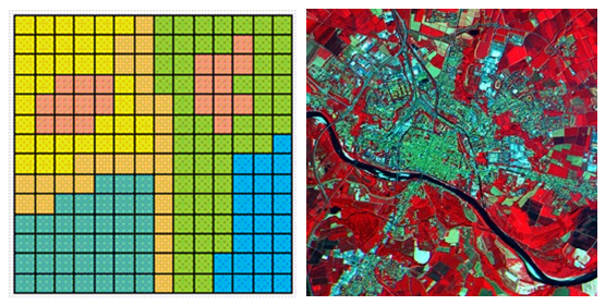
Raster Data

Raster data is the other major format of geographic data. It is made of a grid of equally sized square cells; each cell has an associated value. The most common type of raster data is an image, where the cell value represents the colour that cell should be displayed as.

In the geographic context, the most common raster data is satellite and aerial imagery, although other things can be represented as raster data, for example, population count. A lot of environmental data is provided in raster format, which, in a statistical setting is often used for analysis relating to Sustainable Development Goals and Natural Capital.

Raster data, particularly satellite and aerial imagery, often has large data sizes and can need specialist tools to work with.

Tabular Data

Tabular data is not geographical by default, but often provides information which can link it to a location (for example, coordinates or GSS geography codes).

Look-ups and code lists

Look-ups and code lists provide links between different administrative and statistical geographies, and the GSS codes which relate to each geographic area. For example, our most commonly used lookups link postcode or address to administrative areas (such as Wards, Parishes or Local Authorities). Some look-ups define how different entities nest within or relate to each other in a hierarchy.

These look-ups allow us to easily aggregate data to a huge range of geographies correctly.

Geographic File Formats

Geographic data comes is a range of formats. Most GIS software is good at dealing with these formats, so you shouldn’t worry about them too much. However, there are some pros and cons which you should be aware of as a user.

Shapefiles

• Shapefiles are the most common and long standing file type.
• Shapefiles only store vector data.
• One shapefile requires the following 3 files:
  • .shp - the feature geometry
  • .shx - the shape index position
  • .dbf - the attribute data
  • and there are also optional files like .prj (which stores the projection system information) and .xml (which stores metadata).
• For a shapefile to be valid the files above must be stored in the same directory and have exactly the same file name. If you move a shapefile or send it to someone else make sure you include the .shp, .shx and .dbf files otherwise the shapefile will be corrupted and unusable.
• There are some frustrating quirks when using shapefiles which can cause you problems. Be aware that:
  • attribute names are limited to 10 characters
  • file size is limited to 2GB
  • there is no NULL value which makes distinguishing 0s and NULLs problematic
  • an individual shapefile can only deal with one type of vector data (points, lines or polygons) so you will need multiple shapefiles if you are working with multiple types of vector data
  • by default there is no projection data provided with shapefiles (unless you have a .prj file) so it is up to the user to make sure the data is projected in the correct coordinate reference system. This makes it easy to put data in the wrong place by accident.

GeoPackages

• Geopackages are a modern data format based on an Open Geospatial Consortium standard.
• A geopackage is a self-contained SQLite database which can hold multiple layers.
• Geopackages can hold a range of data types including vectors, raters, tiles and flat formats.
• Using a geopackage can allow you to avoid the problems encountered with shapefiles.
• The geopackage file format is .gpkg.

GeoJSON

• GeoJSON is a version of JSON which is spatially enabled which means locations are stored within the format.
• GeoJSON is a text representation of vector data.
• Like geopackages, GeoJSON is an open standard.
• Location is encoded in GeoJSON as longitude and latitude in WGS84 reference system. As much of the UK’s data is provided in the British National Grid projection you need to take care with this format.

KML and KMZ

• KML and KMZ (the compressed version of KML) are XML representations of vector data.
• These formats are most frequently used in Google Earth, so can be a good way to provide data to a non-GIS user who wants to visualise it easily.
• Again, these formats are an OGC standard.
• Realistically you won’t find much use for these formats as a GIS user, but will occasionally stumble across them.

Locating Spatial Data

Coordinate Systems

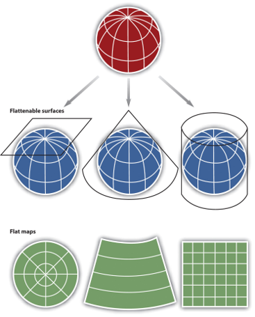
Longitude and latitude are used to represent locations on a 3D globe (the Earth) - this is called a geographic coordinate system.

However, it’s not easy or accurate to complete analysis or measure distances on a globe. So, we use a projected coordinate system instead. A projected coordinate system is a representation of the globe on a flat surface - a map. The trouble with projected coordinate systems is that they aren’t a perfect representation of a 3D object, as anyone who has ever tried to wrap up a ball will know!

Coordinate Reference Systems

In GIS a coordinate reference system (CRS) defines how data is plotted on a projected reference system.

As we mentioned earlier, projected coordinate systems are not a perfect representation of the 3D Earth. To account for this, many different projected coordinate systems have been created which focus on providing a more accurate representation for a smaller area (for example, a continent or country). There are a lot of subtleties and technicalities to coordinate reference systems which you don’t need to worry about. However, you do need to be aware of CRSs to avoid making mistakes in your analysis.

GIS software is good at handling data projected in different CRSs on the fly. This means that when you load two datasets that are projected in different CRSs the GIS will make them appear in the right place relative to each other. If you are only visualising data this is fine.

When you are doing analysis having data in different CRSs will cause errors. So, before you start doing analysis, check the coordinate reference system of all of your data. If your data have differing CRSs, you will need to reproject them to the same CRS before starting analysis.

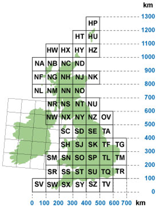
British National Grid

In Great Britain, Ordnance Survey have created British National Grid which is the best CRS for locating land-based data for the British Isles. Almost all of the data you will deal with will come in this CRS.

Some common CRSs

The variables which define CRSs are complex and it’s easy to make mistakes with them. So, CRSs have an EPSG code assigned to them which makes identifying them easier. You can use this EPSG code in all GIS software and coding languages to search and define the CRS you want to use.

These are some of the most common CRSs you will come across and their EPSG codes.

In the UK

• British National Grid
  • EPSG: 27700
  • Covers Great Britain and Northern Ireland
• Irish Transverse Mercator
  • EPSG: 2157
  • Covers Ireland and Northern Ireland
  • There are also some older Irish CRSs in use so take care here.

In Europe

• ETRS89
  • EPSG: 4936
  • Commonly used by Eurostat

Globally

• WGS84 - Mercator
  • EPSG: 4326
  • The ‘standard’ world map
• WGS84 - Web-Mercator
  • EPSG: 3857
  • A specialised version of WGS84 for web mapping.
  • Looks very similar to EPSG: 4326 but is actually different, so take care!

Where to get Geospatial Data

Office for National Statistics

ONS produces a range of geographic data, including boundaries, lookups, directories and classifications.

This data is available for download or access via API from the Open Geography Portal. The ONS Geography Linked Data Portal is a companion site for the Open Geography Portal, and allows you to search for geographical entities or places and understand the different types of geographies available in that area.

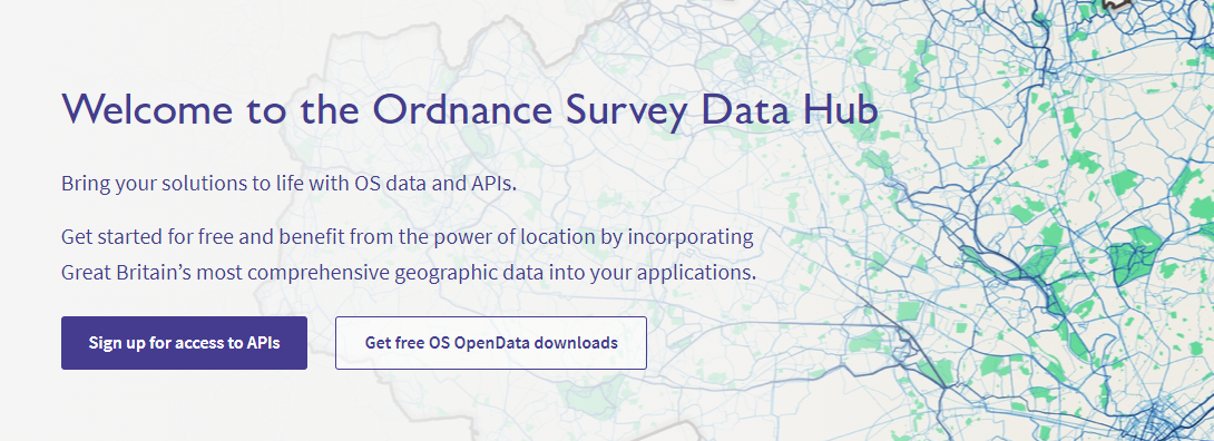
Ordnance Survey

Ordnance Survey provide a wide variety of geospatial data which far exceeds the needs of most statisticians and analysts. Open data as well as premium data available to the Public Sector through the Public Sector Geospatial Agreement (PSGA) can be accessed via the Ordnance Survey Data Hub. We recommend following the excellent tutorials available in the Documentation to get started.

Other Sources

Geographic data is available from a huge range of sources, which we cannot possibly cover in this tutorial. As with all data you should evaluate the quality, provenance and suitability of the data you source.

Features of ONS Geography Products

GSS Names and Codes

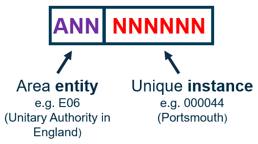
On 1st January 2011 GSS codes were introduced. GSS codes are a type of uniform resource indicator (URI) which provide a way to identify unique items. GSS codes identify individual geographic objects, for example, Local Authority Districts.

GSS codes are comprised of two codes: a three character entity code which describes what type of statistical geography the object is, and a six digit number which refers to the unique instance of the object.

GSS codes can be used to look up specific areas on the ONS Geography Linked Data Portal. This website provides a useful insight into the relationships between statistical geographies across the UK.

The Register of Geographic Codes is the definitive list of all codes in use for UK statistical geographies. It should be used in conjunction with the Code History Database which charts historic changes in codes, which can be useful when understanding how statistical geographies have changed over time.

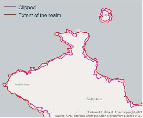
Geographic Extent

ONS creates boundaries at two different extents:

• C: clipped to the coastline (mean high water mark)
• E: extent of the realm (mean low water and offshore islands in some cases)

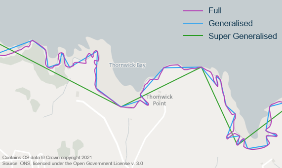
Resolution

Boundaries are made up of a string of point which join together to make a whole polygon. Omitting points in this string can make a more generalised boundary which can be useful when speed and size are important, for example, web mapping purposes.

ONS creates boundaries at four resolutions

• F: full
• G: generalised - 20m
• S: super generalised - 200m
• U: Ultra generalised - 500m

Note that not all resolutions are available for all boundary extents or boundary types.

Combining Resolution and Extent

The extents and resolutions above are combined to produce several different versions of each boundary output, suitable for a range of different uses.

For analysis the most detailed boundary data available (most frequently BFE) should be used to avoid errors. This is particularly important when combining or comparing datasets, or when allocating things using boundaries.

For mapping or visualising your data a more generalised dataset can make outputs easier to interpret and will be quicker to load, improving user experience.

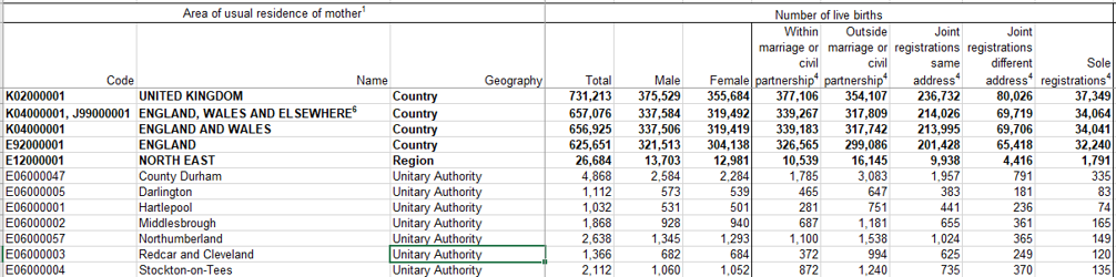
When downloading boundaries from the ONS Geoportal you will find the following codes. This table will help you understand them.

Generalisation	Clipped	Extent of the Realm
Full	BFC	BFE
Generalised	BGC	-
Super Generalised	BSC	-
Ultra Generalised	BUC	-

Overview of ONS Geography Products

ONS produce a range of geographical products for use across a number of organisations and applications. UK geographies can be very complex as they accommodate this range of uses and applications. Administrative boundaries in the UK also change frequently which results in changing and updating boundary datasets. When producing statistics we must be conscious of this to avoid errors.

The Hierarchical Representation of UK Statistical Geographies provides a detailed overview of the different boundaries available and how they are associated with each other. This is a useful resource to refer back to - you can find it on the Open Geography portal

We’ll now run through some of the more frequently used geographies to be aware of.

Administrative Geographies

Regions

• 9 regions in England
• No regions in Scotland, Wales or Northern Ireland.
• For UK wide representation, often England’s regions are shown with the country boarders for Scotland, Wales and Northern Ireland.
• Local Authority Districts (also known as Lower Tier Local Authorities) nest within regions.

Local Authorities

• The Local Government structure in England is a two tier system which creates some complexity. The other UK nations have a single tier system.
• The two tier system means there are two different boundary sets for Local Authorities. Here is how they are made up in 2020:
  • Upper Tier Local Authorities (UTLA)
    • England: 151
    • Wales: 22
    • Scotland: 32
    • Northern Ireland: 11
    • Total: 216
  • Lower Tier Local Authorities (LTLA)
    • England:314
    • Wales: 22
    • Scotland: 32
    • Northern Ireland: 11
    • Total: 379
• Lower Tier Local Authorities (LTLAs) are also known as Local Authority Districts (LADs).
• Local Authority boundaries change frequently so ensure you use the correct year to avoid errors.

Census Geographies

Output Areas

• Census geographies are stable, small area geographies created for non-disclosive census releases.
• These areas represent the nighttime residential population.
• They were introduced in 2001 and revised in 2011 to reflect population changes and better align with administrative units. They will be revised again in 2021.
• The geographies are built from clusters of postcodes which are aggregated to be as socially homogenous as possible, based on a range of factors.
• Each level of geography has a relatively consistent population size.
• Mixtures of urban and rural areas are avoided wherever possible.
• The Census geographies are hierarchical and nest within each other, as shown in the image below.

Workplace Zones

• Workplace Zones are used to publish workplace related statistics
• They are a representation of the workplace population (ie. day time population distribution)

Postcodes, UPRNs and Addresses

Postcodes

ONS produce two postcode directories. Both directories provide information about which area the postcode lies in for a range of different boundary products. However, the directories have subtle differences so make sure you select the correct one based on what you’re using it for.

ONS Postcode Directory (ONSPD)

• Postcodes are assigned to areas via direct point-in-polygon assignment (ie. overlaying postcode points on geographical boundaries to show which area the postcode lies within)
• This method provides a more accurate locational assignment.
• This directory should be used for operational purposes where an accurate postcode location is important.

National Statistics Postcode Lookup (NSPL)

• Postcodes are assigned to Output Areas (OAs) by point-in-polygon assignment. Then, OAs are assigned to other statistical areas by ‘best-fit’ method (more on this later in the course.)
• The best fit assignment can mean the postcode appears to be in the wrong place (but it isn’t).
• This directory should be used for statistical production, where it is important to ensure data is assigned to the correct area within the relevant geographical hierarchy.
• It’s worth noting here that ‘best-fit’ isn’t used for certain geographies, for example, National Parks. If you want to know more about this have a look at ‘An overview of best-fitting’.

Unique Property Reference Numbers - UPRNs

UPRNs are 12 digit reference numbers which are assigned to every addressable location in Great Britain. Addressable locations include buildings and objects like bus shelters and electricity substations.

UPRNs are authoritative codes and can be used for data linkage. At ONS, UPRNs form one of the five frames within the Reference Data Management Framework (RDMF), which enables accurate data linkage.

UPRN Directories

ONS produces two UPRN directories, which are similar to the postcode directories. The UPRN directories provide statistical geography information for each UPRN.

ONS UPRN Directory (ONSUD)

• Created by point-in-polygon assignment of UPRNs to geographic boundaries.
• Provides a more exact location assignment.
• Use for operational purposes.

National Statistics UPRN Lookup (NSUL)

• UPRNs are assigned to output areas via point-in-polygon assignment, and then linked to other statistical geographies by best-fitting.
• URPNs can appear to be in the wrong place, but they aren’t.
• Use this directory for statistical production.

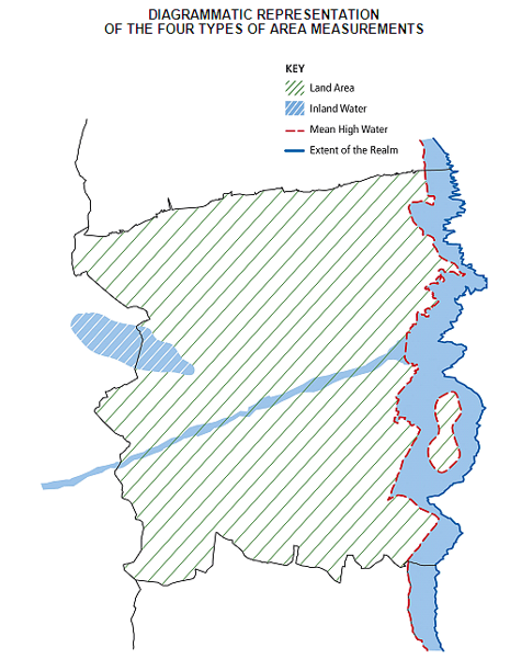
Standard Area Measurements

Standard area measurements are official measures for the area of geographic entities. They should be used whenever you are doing a calculation which uses area as a factor (eg. calculating population density).

There are a number of types of standard area measurement which reflect different measures of the coastline and inland water. AREALHECT is the measure that is most often used, and is recommended for use when calculating statistics like population density, but you may find that the other measures are appropriate for other applications. Their definitions are available below and more information is available in the User Guide.

Definitions of the Types of Standard Area Measurement

Measure	Definition
AREAEHECT	Area measurement to extent of the realm boundaries (mean low water mark) in hectares.
AREACHECT	Area measurement to coastline feature boundaries (mean high water mark) in hectares.
AREAIHECT	Area measurement of inland water features larger than 1km2.
AREALHECT	Area measurement of land area only (to coastline features and excluding inland water features larger than 1km2).

Rural-Urban

There are multiple methods for defining “urban” and “rural”. Two of the most common are the Rural Urban Classification (RUC) and Built-up Areas (BUAs).

Built-up Areas are defined geospatially using a 50m x 50m grid which covers the country. Each cell is classified using Ordnance Survey’s MasterMap topography data; the cell is defined as built up if over a certain proportion is covered by man-made features. When a large enough area of contiguous built-up cells is reached, that area is defined as a built-up area. Built-up areas are not strictly urban but rather developed.

Rural Urban Classification has a common demographic definition. Urban is defined as an area where >50% of the population belong to a built-up area with a population >10,000. This classification also includes categories such as sparse and non-sparse, according to the population density profile of an area.

Other methods of defining rural-urban are often adjusted versions of BUAs which comply with different boundary types (for example. major towns and cities).

Area Classifications

Area classifications are an analysis of people by where they live. Areas can be classified by the characteristics and attitudes of those who live in them. This is based on the concept that similar people with similar characteristics are more likely to live within the same locality. These area types will be distributed in different geographical space.

The Output Area Classification (OAC) is a commonly used area classification derived from Census data. You can investigate the 2011 OAC via this interactive map.

An interim 2021 Output Area classification for England and Wales has been produced as a collaboration between the ONS and University College London.

A UK classification, keeping the same supergroups, groups and subgroups is planned which will include 2021 Census data for Northern Ireland and 2022 Census data for Scotland.

Geospatial Tools

Open Source

There are many excellent open source geospatial resources and tools available. We would specifically recommend the following:

QGIS is a desktop GIS tool which will allow you to quickly load and visualise your data. This software is used by geospatial experts across the world and is the leading free and open source GIS software. If you want to use geospatial data and don’t know how to code, this is a great way to get started. Take a look at our Introduction to QGIS training for a walkthrough of tasks you might end up doing in a statistical context. To install QGIS at ONS you will need to request it via Service Desk; after approval install can be completed via the software centre.

Python users can make use of GeoPandas for manipulating spatial objects; GeoPandas is the spatial version of Pandas so you should find it familiar. For mapping we recommend using matplotlib and for raster analysis we recommend rasterio. If you work at ONS you’ll find installation of geospatial Python packages slightly awkward so follow our installation guidance to get going. Our Introduction to GIS in Python training will help you get started with geospatial Python.

R users will find sf the best option for manipulating spatial objects; sf integrates well with the tidyverse so should be comfortable for many R users. There are a number of mapping packages, we recommend tmap for its simplicity, but ggplot2, cartography and leaflet are also excellent options. For raster data we recommend using raster or stars. At ONS these packages are all available to install via the Artifactory, as usual. If you’ve never used geospatial R packages then you might find Introduction to GIS in R a good place to start.

Proprietary Software

There are some popular pieces of proprietary software for geospatial applications.

ArcGIS (including ArcMap and ArcGIS Pro) - a desktop GIS software similar to QGIS.

FME an ETL software which can be useful for automating processes, including geographic ones.

At ONS we have licences for these software, although they are generally used by Geographers working in Data Architecture. You should contact the Geospatial team if you need access to them.

Geospatial Analysis Techniques

Basic Spatial Analysis Techniques

This section will give you an overview of some of the most commonly used spatial techniques available in GIS, which can be used to answer numerous questions around location. While the techniques outlined in this section are simple, they are very powerful when combined and can aid you in answering complex analyses. Developing a solid understanding and practical foundation in these techniques will take you far geospatially and will serve as a good base to build more complex skills. Our training walkthroughs in QGIS, R and Python cover how you can undertake these techniques.

A quick reminder: don’t use these techniques to modify statistical or administrative boundaries without thinking about what you are doing carefully - check the GSS Geography Policy on managing change for more details.

Joining data to boundaries

While not strictly a spatial analysis technique, joining tabular data to spatial data is often the first step of analysis you will undertake.

Tabular data which has a GSS code can be joined to any ONS boundaries by this code. As with any join, care should be taken to ensure the join is successful. If nothing joins then you may be using the wrong boundaries so check you have the right ones. If some rows join correctly but others done then check your geographical coverage (you may be joining data and boundaries with different extents, eg. GB data to UK boundaries) and the publication date of your data and boundaries (you may be joining data to boundaries which have different codes in areas due to boundary changes).

Point in Polygon is a way to join point and polygon feature attributes together, by joining points which fall within the polygon boundary. For example, this is frequently used to aggregate points to statistical geographies. Point in polygon is used to create the ONS postcode directory and national statistics UPRN directory; this method is used to assign the postcode or UPRN to the statistical geographies. The attributes of the points will be assigned to the polygon.

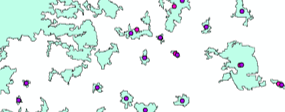
In this example we have joined the points to the green areas they fall within

Select By Location allows you to select features based on their location relative to other features.

There are a number of different spatial relationships, or predicates, which you can use to select by location, for example:

• features which intersect
• features within another feature
• features which touch another feature

This documentation explains the predicates and how they work for the different vector data types.

Selecting by location is an incredibly useful tool and is frequently used across a range of geospatial contexts. For example, to find out how many homes are affected by flooding you can select homes which fall within the flood boundary. You can also combine a number of different selection techniques to answer queries which include more than one variable, for example, selecting homes which fall within a flood boundary and touch the 10 meter contour line.

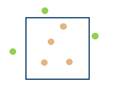
In this example we have selected all the points which fall within the blue square; the selected points are in orange

Buffer allows you to calculate the area a certain distance away from an object. It can be undertaken on all three vector data types and raster data. While most buffers are calculated outwards from the object, you can use negative buffers for polygons which are useful when considering an area inside a polygon.

To find households within a certain distance from a GP surgery, for example, you would buffer the surgery’s location and then (using select by location) select the households which fall within the buffer.

In this example we have buffered the blue features. The resulting buffer is the green feature.

Dissolve allows you to merge together polygons which overlap. This can be useful when considering two overlapping areas as one, when you want to avoid double counting the overlapping area.

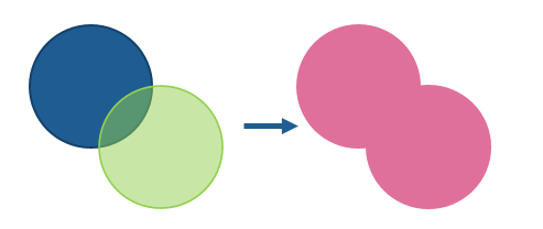
In this example the blue and green polygons have been dissolved into one object - the pink polygon

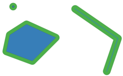
Clipping uses the extent of one geographic feature to trim another feature by. For example, if you have a land use layer for the entire country, but were only interested in one region, you could clip the land use layer to the region boundary and would be left with land use for that region. By removing irrelevant data, this tool can speed up analysis and improve the focus of visualisations.

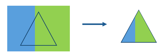
In this example the blue and green layer has been clipped to the triangular feature

Merge combines two or more layers into a single layer. It’s different from dissolve as features which overlap are not combined into one feature but are kept as separate, overlapping features. This tool can be used to bring separate datasets together while still maintaining the individual features within the datasets.

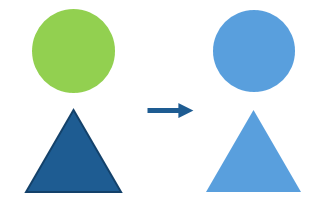
In this example the blue and green layers are merged, resulting in the lighter blue layer

Advanced Analysis Techniques

The basic techniques outlined above can be easily utilised and have the power to provide great insights into statistical data. However, there are more complex techniques and data sources which can be used to provide more detail or statistical rigour to analyses. It is worth being aware of these techniques, although we would not expect you to be using them without more support or training.

Networks, drivetime and zoning can be used to solve problems relating to networks. One of the most commonly used networks is the road network, which allows you to answer questions like “how far is it to drive between these two points?”, “how far from this point can I travel in 30 minutes?” or “what areas can a field staff member cover in 1 hour of driving?”. Network analysis has been successfully used to plan field staff areas for the Census.

This map shows average travel time zones to the ONS Titchfield office. It has been calculated using the Ordnance Survey Highways network and shows the average time it takes to travel to the office in light traffic.

Cluster and Hotspot Analysis can be used to expose spatial groups or patterns which may not be visible to the human eye, particularly when dealing with large datasets. Statistical cluster analysis aims to classify or group objects into a number of different clusters, based on measured variables. This allows clustering of objects based on similarity (often in multiple dimensions) and location.

These methods can add statistical rigour to analysis, allowing us to express measures of statistical confidence based on the patterns or groups that are observed.

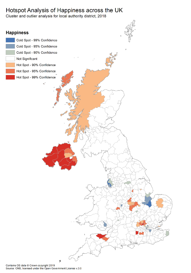
This map shows the results of hotspot analysis for happiness data from 2018. It shows significant clusters of high happiness (hotspots shown in red) and low happiness (cold spots shown in blue).

Earth observation and machine learning are often combined to analyse satellite data. Analysis of satellite data is a complex field that exists in its own right. So, for statistical applications, we tend to use data derived from satellite data to complement our analysis. For example, machine learning can be used to extract building outlines which can then be analysed using techniques outlined earlier.

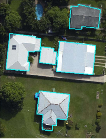
An example where machine learning has been used to extract building outlines from satellite data.

Mapping your data

Mapping your data is one of the most powerful things you can do with GIS. Maps are excellent tools to effectively present results, but can also be useful when interrogating source data or investigating potential relationships and patterns. Mapping can also be a useful QA tool which allows you to identify anomalies and spot errors.

Any GIS will give you access to a range of map types and will allow you to customise the design of your map through adjustable ranges, colour schemes and symbology. These will allow you to bring your data to life. However, as with any visualisation, you need to think carefully about what you are presenting to avoid misleading. People like and intuitively understand maps, but it is easy to lie with them if you make the wrong design decisions. So, here are a few important features to consider.

Normalising Data

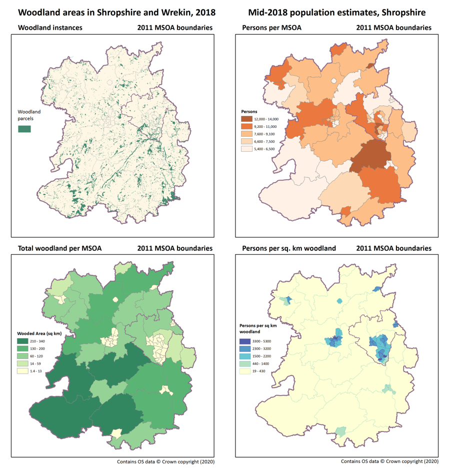
When mapping counts to areas it’s important to normalise your counts. Large areas naturally tend to have larger counts, so it can be misleading to plot raw counts, as large areas tend to dominate the map. By normalising your data (for example, by area) you get a value which is comparable across different sized areas.

In the image below you can see how the raw count of woodland area (top left) can dominate when mapped by MSOA (bottom left). However, when we normalise woodland area by people per MSOA (top right) the resulting map (bottom right) is much clearer, and highlights places of interest where there is a high area of woodland per person.

Selecting Breaks

A choropleth map is a type of map where areas are coloured based on the normalised data value relating to the area. When producing choropleth maps it’s important to select class breaks (sometimes known as bins) carefully, as differing methods of selecting breaks and the number of breaks you choose can significantly change your visualisation. There isn’t a right or wrong method for selecting breaks; ensure your breaks suitably illustrate your data and highlight important features but avoid misleading by hiding data or manipulating breaks to suit your narrative. The image below illustrates how different methods for selecting breaks can drastically change your visualisation.

More Cartography

Cartography is a huge field which we have barely scratched the surface of here. If you’re interested in learning more, keep an eye out for our upcoming training on ‘How to make a good map’.

Geographical Fallacies

There are a number of geographical fallacies which you can fall foul of when undertaking geospatial analysis. Be aware of these to avoid making mistakes in your work.

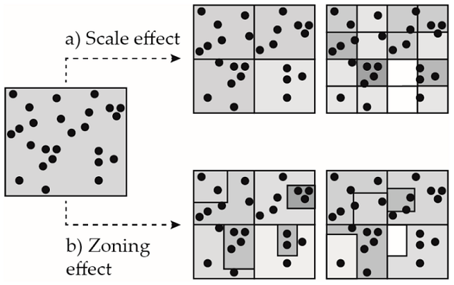
Modifiable Areal Unit Problem (MAUP)

The modifiable areal unit problem (MAUP) is a common source of statistical bias in geographic data where points are aggregated to areas. MAUP is where the same underlying point data can yield different statistical results when aggregated to areas of different size or shape. Statistics can easily be manipulated by changing the geography used. Gerrymandering is a common example of MAUP that you may be familiar with.

As much of the statistical data we deal with is aggregated from point data, we have to be particularly careful of this problem. Using consistent boundaries is the main way we avoid MAUP; this is why change management is one of the pillars of the GSS geography policy, and also why you should avoid creating your own boundaries or modifying existing ones.

Locational Fallacy

Locational fallacy is caused by the spatial characterisation of events in a simplistic or incorrect way. This characterisation can subsequently influence the understanding of the subject and can lead to incorrect outcomes or understanding.

For example, recording locations for all crimes can be misleading. Crimes like burglary or assault occur at a location, so it is suitable to associate these crimes with a location. However, allocating crimes like fraud to a location is less straightforward as it can be committed virtually as well as in person. Incorrectly assigning a crime like fraud to a location can cause misunderstandings in how and why fraud victims are targeted.

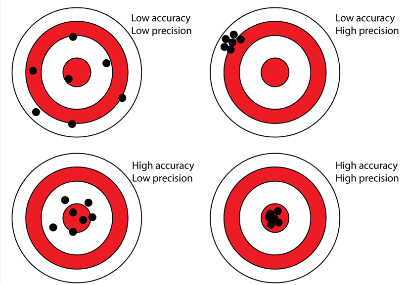
Accuracy and Precision

Accuracy and precision are important to appreciate in order to understand potential bias or errors within your data.

Accuracy is how close a piece of data is to the real-world value.

Precision is how exact the measurement of the data is.

Accuracy and precision can refer to both the object being measured and its location.

A common example of mistakes with accuracy and precision in a spatial context is to provide locational precision to a very high level (mm or even smaller) in a GIS or map, when the location of the data was measured with a GPS which had an error of +/-3 meters.

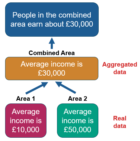
Ecological Fallacy

Ecological fallacy is where incorrect inferences are drawn about an individual based upon information data from a group they are in. For example, a high crime rate in a deprived area does not mean that poor people are criminals.

Aggregating data can conceal variations within an area - the diagram below shows an example of this.

Conclusion

Congratulations on reaching the end of the course.

By now you should have a good understanding of the theory that underpins geospatial analysis. We have covered:

• Geographic data
  • types
  • file formats
  • coordinate reference systems
  • where to get data
• ONS’s geographical products
• Geospatial tools
• Geospatial analysis techniques
• How to visualise your data
• Geographic fallacies to avoid

Now it’s time to apply your newly gained knowledge. Take a look at our practical modules to learn how:

• Introduction to QGIS
• Introduction to GIS in R
• Introduction to GIS in Python